This is a brief tutorial showing how to use differential equations to do make predictions about the state of a simple dynamic analogue electronics circuit. I have ported this post over from my discontinued Wordpress blog, as some readers may find the information useful.

Put simply, a differential equation is any equation that contains derivatives. A derivative is basically a gradient, and so it is an equation that describes a system containing something that changes. In audio, this will likely be something that changes over time (t), so an example might be

I looks kinda like a polynomial, but with various order derivatives. We’d call this example a second order differential equation, as the highest order derivative is 2.

I quickly want to move onto a real world example, showing some useful stuff we can do with differential equations. For this, I’m going to use simple electronic components in a circuit and then try and predict the state of the circuit at a given time. I’m going to use basic analogue electronic components for my first real-world example, as digital filter theory is rooted in basic analogue electronics theory.

The complex impedance ($Z$) of a circuit is made up of real resistive terms ($R$) and imaginary reactive terms ($X$) …

The reactance term comes from the combination of inductance and capacitance. Like resistance, capacitance and inductance are inherent properties of electronic components. The capacitative effect comes from built up electric field that resists voltage changes. The inductive effect comes from the build up of magnetic field that resists changes in current. Reactance effects are only exhibited when circuit conditions change. Therefore, we can use differential equations to predict the state of a circuit after a change. For the following example, the change is the circuit being switched on.

Consider a simple circuit containing a prefect voltage source, a resistor and an inductor …

When the circuit is switched on, the inductor chokes the initial burst of current, giving rise to a gradual increase in current through the inductor until a maximum value is reached.

One way to visualise the current flow through this circuit is to build it and measure it, but this is a bit of a faff. Another way is to use electronic simulation software. For simple circuits (and even for relatively complex ones too) I am a huge fan of the excellent and free web app, CircuitLab. CircuitLab allows the user to just drag and drop various components, set their values, then produce simulation plots like that shown below.

The plot shows that the rise in current through the inductor is not linear with time. This is because the relationship between the inductance (L), voltage (V), and current (I) is differential - it changes over time …

We will now see if we can predict the current for any given time analytically using differential equations. We know from Kirchoff’s Voltage Law that the sum total voltage drop across series components (VR and VL) equals the supply voltage (VS) …

We want to predict the current, so using Ohm’s law (V=IR), we can express this in terms of current (I) …

The next thing we want to do is get this into a suitable form for integration so we can remove the differential terms (dI and dt) and find a solution. THe first step is to split dI and dt …

… then separate the rest of the variables …

This is now in a suitable form for integration.

This is a great time to introduce a web app that I find particularly useful, Wolfram Alpha. This tool can be used to perform calculus. It will show the intermediate steps towards a solution, so there is no black-box trickery to get in the way of our understanding. I have posted a screenshot of the output of the web app when asked to integrate the left-hand-side (LHS) of the above equation. It saves all the $LaTeX$ typing anyway!

Integration of the right-hand-side (RHS) is trivial, so we end up with the following …

We are still trying to solve this for current, so the next step is to isolate the logarithmic term so that both sides of the equation can be easily exponentiated …

Now simply exp() both sides …

Now save a little writing by using the following alias for K, where K is some constant term …

… and so …

This allows us to finally get the current term by itself …

Great! We can almost state the current at a given time after the circuit is switched on, but there are still some pesky unknown constant terms in K that would cause some uncertainty in the result. However, this is not a problem because we know the initial conditions at switch on. At time t=0, the current through the circuit I=0. Substituting this in …

And so it follows …

so …

Now we can determine the current at any given time after switch on!

It is then easy to check if our analytical solution matches our hardware equivalent by making a quick Matlab script …

1
2
3
4
5
6
7

tAxis = 0:1e-4:5e-3; % Time Axis

% We can use a Lambda to neatly represent our solution
current = @(V,R,L,t)(V/R)*(1-exp(-t*R/L));
figure;
plot(1000*tAxis,1000*current(9,20,10e-3,tAxis),'Linewidth',2);
xlabel('Time [ms]'); ylabel('Current [mA]'); ylim([0 500])

So there we have it. I differential equation solved that allows us to predict the behaviour of a real physical system.

I’ve always liked the ability to rapidly profile code snippets in Matlab using the ‘tic’ and ‘toc’ commands. I wanted to develop something equally as simple to use in C++ for rapid tests. It turns out that a particularly elegant way to do this is to use RAII techniques, allowing easy profiling of any commands within a scope. A time marker is made on construction, and another time marker is made on destruction, and then compared to the original time marker.

The new ‘chrono’ classes bundles in the C++11 standard library make this task particularly simple. Below is the full class for simple tic toc type profiling …

1
2
3
4
5
6
7
8
9
10
11
12
13
14
15
16
17
18
19
20
21

// TicToc RAII profiler
class TicToc
{
private:
    typedef std::chrono::high_resolution_clock clock;
    typedef std::chrono::microseconds res;
    clock::time_point t1, t2;

public:
    TicToc() {
        t1 = clock::now();
    }

    ~TicToc()
    {
        t2 = clock::now();
        std::cout << "Elapsed time is "
        << std::chrono::duration_cast<res>(t2-t1).count()/1e6
        << " seconds.\n";
    }
};

Putting this to use is very simple. Just make a new scope using the scope resolution operator and create an instance of TicToc. When it goes out of scope, it will be deleted from the stack and will display the elapsed time.

1
2
3
4
5

{
    TicToc t;
    someFunctionToProfile();
    perhapsSomethingElse();
}

Furthermore, other classes can be derived from this simple class, making this a really simple way to get stats on object lifetime.

Enjoy and HAPPY NEW YEAR!

An interesting question popped up on stackoverflow about palindrome detection in c++. A palindrome is a word whose characters can be reversed, and no change is detectable, e.g. “racecar”. My initial thought was to make a copy and use the std::reverse algorithm …

1
2
3
4

tupni = input;
std::reverse(tupni.begin(), tupni.end());

if(tupni==input){ ...

However, this copy can be avoided using reverse itterators . .

1
2
3
4
5
6

bool isPalindrome(const std::string& str)
{
    // comparison based on 2 string iterators - a "normal" one
    // and a reversed one
    return std::equal(str.rbegin(), str.rend(), str.begin());
}

Seeing as this function only contains a single command, it might be nice to use a lambda as an alternative. You can specify a return type from a lambda with this syntax

1

[]()->return_type{}

So defining the palindrome detector becomes a simple 1-liner.

1
2
3

auto isPalindrome = [](const std::string& str)->bool{return std::equal(str.rbegin(), str.rend(), str.begin());};
std::cout << isPalindrome("racecar") << std::endl; // prints 1
std::cout << isPalindrome("truck") << std::endl; // prints 0 

I will start posting cool little blocks of code, like short poems when I see neat little things to do ..

1
2
3
4
5
6
7
8
9
10
11
12
13
14

#include <iostream>
#include <vector>
using namespace std;

int main ()
{
	vector<int> v{12,324,45,65,787,9}; //Uniform initialization
	cout << "In vector: ";
	for (auto val : v) {cout << val << ", ";} //Range based for
	int m = 5;
	cout<< "there are "
		<< count_if(v.begin(), v.end(), [m](int i){return i%m == 0;}) //lambdas
		<< " multiples of " << m << endl;
}

In vector: 12, 324, 45, 65, 787, 9, there are 2 multiples of 5

For some more depth on the functional goodness see this Dr. Dobbs article

Using inkscape vector graphics to generate a website logo

This is a quick tutorial showing the steps required to generate a logo like the one seen at the top of this page. For this, I used the fantastic open source Inkscape software. In the past, I have tried to learn how to use various vector graphics drawing software packages, but have always run out of patience. This was until trying Inkscape. In comparison, Inkscape is easy to grasp and there is a large amount of user generated documentation online that will help you to produce amazing looking graphics in no time.

I am an inkscape beginner but thought it might be useful to produce a brief tutorial that combines some of the basic techniques that I’ve leant from other tutorials. I have noticed that many of the tutorials on the web do not take good advantage of the layers tools and so I hope to address this here. This tutorial was generated on a mac and so the screenshots have a mac look and feel. However, the commands outlined here should be identical on all platforms.

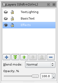
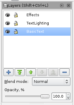
The first step is to open up the layers menu widget (Shift+… as shown) thing. I decided that I wanted some text with some lighting to make it look shiny and some special effects like a glow and a shadow. I decided to break this idea down into three layers as shown in the screenshot.

The next step was to create a basic logo using the text tool. Do this on the ‘BasicText’ layer. The ‘AP’ part of the logo used a non-standard font downloaded from a free font website. The colours of the text can be changed easily by highlighting a selection and then selecting one of the colours from the swatch at the bottom of the Inkscape window.

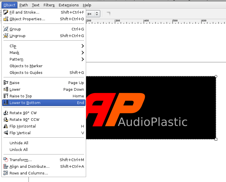
I wanted to check that the text was legible when using a black background. For this, I created a black rectangle and sent it too the back by using the item shown in the object dropdown menu. All looks good so I deleted the black box.

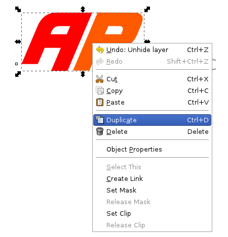
The next thing that I wanted to do was add lighting effects. I was only interested in doing this on the large text. The first thing to do was to duplicate the target text.

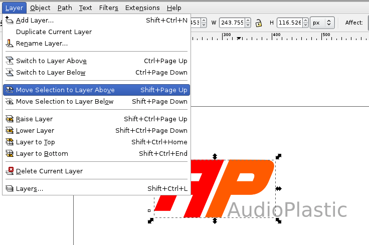
Once the duplicate was created, I moved the duplicate to it’s own layer that I reserved earlier for lighting effects.

The visibility of each layer can be changed by clicking the eye image in the layers menu window. The fist job that I did with the duplicate was to create a gradient from black to transparent, from bottom to top. THis was to make the lower part of the text look as if it is in a relatively shaded region The gradient can be locked to the vertical plane by holding the ctrl key while dragging the gradient tool.

<img src=”/images/inkscape_logo_tut/Screen shot 2011-07-02 at 08.24.46.png” width=100%>

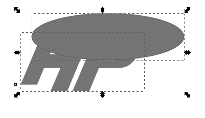
The next idea was to make the top of the text look shiny, like light is coming from above. For this, another duplicate was made and pushed into the lighting layer. I coloured it grey for better visibility. I then put an elipse on top of this duplicate.

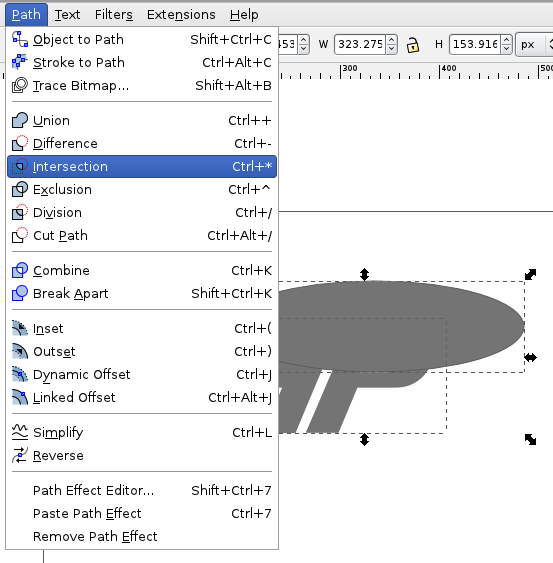
The elipse and duplicated text were both selected and the intersection tool in the path menu was then used.

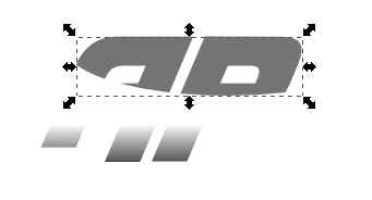
This does what it says on the tin.

Setting the basic text layer to visible under this gives the following.

The colour of the inset was changed from grey to white and then a gradient was applied to transparent, adding to the shiny look.

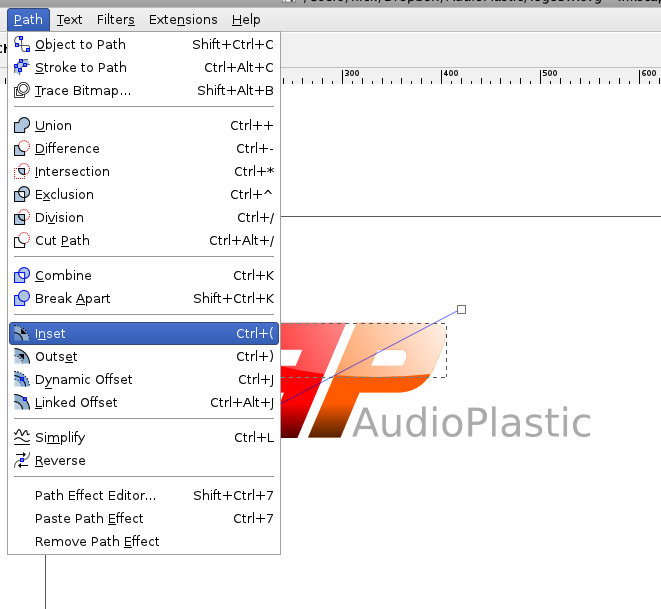
To give the edge of the text more colour definition, an inset was added like so.

To give the following result.

Looking good! I wanted to give the coloured text a neon glow, so I duplicated the basic text once more and pushed it into the effects layer.

I then used the blur tool from the colours window to get the glow effect.

<img src=”/images/inkscape_logo_tut/Screen shot 2011-07-02 at 08.36.02.png” width=100%>

The layers can all be set to visible once again to see the combined effect.

I again wanted to test the legibility of the text on a dark background after making the lighting and glow modifications. However, instead of just drawing a rectangle and sending it to the bottom of the layer, I created a new later called ‘Alternative Background’, moved that layer to the bottom and then placed the black background within it. This makes switching the background on and off using the layers menu very easy.

<img src=”/images/inkscape_logo_tut/Screen shot 2011-07-02 at 08.40.12.png” width=100%>

In doing this, I noticed that the bottom, shaded part of the text did not contrast well against the background. To rectify this, I went tot the lighting layer and added an inset to the shading.

<img src=”/images/inkscape_logo_tut/Screen shot 2011-07-02 at 08.41.21.png” width=100%>

The resulting image after this transform is much sharper to the eye.

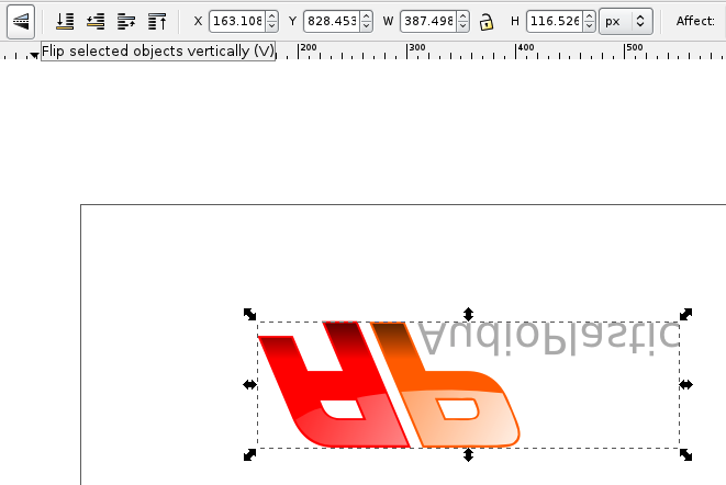
After this, I wanted to create a reflection in the horizontal axis, making the logo appear as if it is hovering above a reflective surface. For this, I created a duplicate of everything, copied it into an new reflection layer, and then flipped the duplicate upside down using the button in the top-left of the following screen shot.

The duplicate was then moved below the original. Holding the ctrl key while dragging only allows the object to move in one dimension, thus making alignment simple.

Colour and transparency were modified.

Glow colour, glow amount and other subtle changes were made

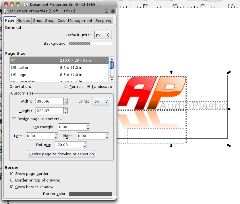
The final image was then ready for export. The first stage in this action was to resize the canvas. In the image properties box, there is a useful too to resize the canvas to mathc the size of the current selection. Seeing as nearly half the selection was transparent in the example shown, the lower margin was tapered in by some pixels

To export the logo in a useful format such as png, use the “export to bitmap” option in the file menu. the first time that I attempted this action, I used the “save as” option to save the image as a png. However, in doing this, I lost all of the alpha information and so the transparency was all messed up. The “export to bitmap” method gives predictable results.

The final png is shown in the operating system preview pane.

The Matlab publishing tool and Jekyll combined

I am in the middle of generating a set of tailored Matlab tutorials for a colleague. We decided that the best way to communicate the work was by using Matlab’s integrated publishing facility. This is a great tool that allows you to generate HTML pages directly from Matlab scripts. Code is highlighted nicely and screenshots of any figures generated are linked in the generated HTML.

I am also a massive Dropbox fan. This is a file synchronisation service that can act as a static website server. Dropbox has a public folder. The Matlab generated HTML can be dropped into this folder and then the public link to the file can be shared. This makes for a very neat and straight forward way to distribute Matlab published documents. However, there are a couple of very minor drawbacks. Firstly, the static html hosting service provided by Dropbox is more of a side effect of the public folder than a supported service. Dropbox makes no guarantees about service uptime or reliability. This would probably never be a problem for the scenario outlined here, but seeing as I generate this site using Jekyll(https://github.com/mojombo/jekyll/wiki) and host it at Github, I thought I would try to combine the two.

This turns out to be incredibly simple. All you need to do is copy the “HTML” folder generated by Matlab into the root directory or any new subdirectory of your Jekyll project. You can then just add the YAML Front matter to the top of the HTML file. In my case the following …

---
layout: main
title: Tutorial xyz
---

… and then Jekyll will render the Matlab published document in your site. The problem is that the Matlab HTML file will likely override some of your own CSS, and so the formatting may be a little off. However, this is very simple to rectify. In my case, I just deleted the following block of code.

body {
  background-color: white;
  margin:10px;
}

h1 {
  color: #990000; 
  font-size: x-large;
}

h2 {
  color: #990000;
  font-size: medium;
}

/* Make the text shrink to fit narrow windows, but not stretch too far in 
wide windows. */ 
p,h1,h2,div.content div {
  max-width: 600px;
  /* Hack for IE6 */
  width: auto !important; width: 600px;
}

I left the rest in, as I quite like he Matlab code formatting. It differentiates the code blocks in the Matlab pages from the code blocks in the blog. If you don’t want to give the mathworks any free advertising you can remove the following too.

<p class="footer"><br>Published with MATLAB&reg; 7.10<br></p>

Happy static site generating!